Asynchronous Successive Halving and Hyperband

Early Stopping


Learning Curves (image from Aaron Klein)

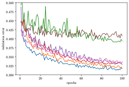
In the methods discussed above, we train each model for 81 epochs before scoring it. This is expensive, it can take up to 1.5 hours. In order to figure out whether a configuration is pretty poor, do we really need to train it all the way to the end?

At least for most neural network training problems, the validation error after training only a few epoch can be a surprisingly strong signal separating the best from the worst configurations (see figure above). Therefore, if a certain trial shows worse performance after (say) 3 epochs than many others, we may just as well stop it early, allowing the worker to pick up another potentially more rewarding task.

Synchronous Successive Halving and Hyperband

Successive halving is a simple, yet powerful scheduling method based on the idea of early stopping. Applied to our running example, we would start 81 trials with different, randomly chosen configurations. Computing validation errors after 1 epoch, we stop the 54 (or 2/3) worst performing trials, allowing the 27 (or 1/3) best performing trials to continue. This procedure is repeated after 3, 9, and 27 epochs, each time the 2/3 worst performing trials are stopped. This way, only a single trial runs all the way to 81 epochs. Its configuration has survived stopping decisions after 1, 3, 9, and 27 epochs, so likely is worth its running time.

In practice, concurrent execution has to be mapped to a small number of workers, and successive halving is implemented by pausing trials at rung levels (i.e., after 1, 3, 9, 27 epochs), and then resuming the top 1/3 to continue training until the next rung level. Pause and resume scheduling is implemented by checkpointing. We will ignore these details for now, but come back to them later. Ignoring practical details of scheduling, and assuming that training time per epoch is the same for each trial, the idea behind successive halving is to spend the same amount of time on trials stopped after 1, 3, 9, and 27 epochs, while making sure that at each rung level, the 2/3 worst performers are eliminated.

Successive halving has two parameters: the reduction factor (3 in our example), and the grace period (1 in our example). For a reduction factor 2, rung levels would be 1, 2, 4, 8, 16, 32, 64, and we would eliminate the 1/2 worst performers at each of them. The larger the reduction factor, the fewer rung levels, and the more aggressive the filtering at each of them. The default value in Syne Tune is 3, which seems to work well for most neural network tuning problems. The grace period is the lowest rung level. Its choice is more delicate. If set too large, the potential advantage of early stopping is lost, since even the worst trials are trained for this many epochs. If set too small, the validation errors at the lowest rung level are determined more by the random initial weights than the training data, and stopping decisions there will be arbitrary.

Hyperband, a generalization of successive halving, eliminates the grace period as free parameter. In our example above, rung levels were [1, 3, 9, 27, 81], and the grace period was 1. Hyperband defines brackets as sub-sequences starting at 1, 3, 9, 27, 81, of size 5, 4, 3, 2, 1 respectively. Then, successive halving is run on each of these brackets in sequence, where the number of trials started for each bracket is adjusted in a way that roughly equalizes the total number of epochs trained in each bracket.

While successive halving and Hyperband are widely known, they do not work all that well for hyperparameter tuning of neural network models. The main reason for this is their synchronous nature of decision-making. If we think of rungs as lists of slots, which are filled by metric results of trials getting there, each rung has an a priori fixed size. In our successive halving example, rungs at r = 1, 3, 9, 27, 81 epochs have sizes 81 / r. Each rung is a synchronization point. Before any trial can be resumed towards level 3, all 81 trials have to complete their first epoch. The progress of well-performing trials is delayed, not only because workers are idle due to some trials finishing faster than others, but also because of sequential computations (we rarely have 81 workers available). At the other extreme, filling the final rung requires a single trial to train for 54 epochs, while all other workers are idle. This can be compensated to some extent by free workers running trials for the next iteration already, but scheduling becomes rather complex at this point. Syne Tune provides synchronous Hyperband as SynchronousHyperbandScheduler. However, we can usually do much better with asynchronous scheduling.

Asynchronous Successive Halving

An asynchronous scheduler needs to be free of synchronization points. Whenever a worker becomes available, the decision what it should do next must be instantaneous, based on the data available at that point in time. It is not hard to come up with an asynchronous variant successive halving. In fact, it can be done in several ways.

Returning to our example, we pre-define a system of rungs at 1, 3, 9, 27 epochs as before, and we record metric values of trials reaching each rung. However, instead of having fixed sizes up front, each rung is a growing list. Whenever a trial reaches a rung (by having trained as many epochs as the rung specifies), its metric value is entered into the sorted list. We can now compute a predicate continue which is true iff the new value lies in the top 1/3.

There are two variants of asynchronous successive halving (ASHA), with different requirements on the backend. In the stopping variant, a trial reaching a rung level is stopped and discarded if continue = False, otherwise it is allowed to continue. If there is not enough data at a rung, the trial continues by default. The backend needs to be able to stop jobs at random times.

In the promotion variant, a trial reaching a rung level is always paused, its worker is released. Once a worker becomes available, all rungs are scanned top down. If any paused trial with continue = True is found, it is resumed to train until the next rung level (e.g., a trial resumed at rung 3 trains until 9 epochs): the trial is promoted to the next rung. If no paused trial can be promoted, a new one is started from scratch. This ASHA variant requires pause and resume scheduling. In particular, a trial needs to checkpoint its state (at least at rung levels), and these checkpoints need to be accessible to all workers. On the other hand, the backend never needs to stop running trials, as the stopping condition for each training job is determined up front.

Scripts for Asynchronous Successive Halving

In this section, we will focus on the stopping variant of ASHA, leaving the promotion variant for later. First, we need to modify our training script. In order to support early stopping decisions, it needs to compute and report validation errors during training. Recall traincode_report_end.py used with random search and Bayesian optimization. We will replace objective with the following code snippet, giving rise to traincode_report_eachepoch.py:

traincode_report_eachepoch.py (relevant part)

def objective(config):
    # Download data
    data_train = download_data(config)
    # Report results to Syne Tune
    report = Reporter()
    # Split into training and validation set
    train_loader, valid_loader = split_data(config, data_train)
    # Create model and optimizer
    state = model_and_optimizer(config)
    # Training loop
    for epoch in range(1, config["epochs"] + 1):
        train_model(config, state, train_loader)
        # Report validation accuracy to Syne Tune
        accuracy = validate_model(config, state, valid_loader)
        report(epoch=epoch, accuracy=accuracy)

Instead of computing and reporting the validation error only after config['epochs'] epochs, we do this at the end of each epoch. To distinguish different reports, we also include epoch=epoch in each report. Here, epoch is called resource attribute. For Syne Tune’s asynchronous Hyperband and related schedulers, resource attributes must have positive integer values, which you can think of “resources spent”. For neural network training, the resource attribute is typically “epochs trained”.

This is the only modification we need. Curious readers may wonder why we report validation accuracy after every epoch, while ASHA really only needs to know it at rung levels. Indeed, with some extra effort, we could rewrite the script to compute and report validation metrics only at rung levels, and ASHA would work just the same. However, for most setups, training for an epoch is substantially more expensive than computing the validation error at the end, and we can keep our script simple. Moreover, Syne Tune provides some advanced model-based extensions of ASHA scheduling, which make good use of metric data reported at the end of every epoch.

Our launcher script runs stopping-based ASHA with the argument --method ASHA-STOP. Note that the entry point is traincode_report_eachepoch.py in this case, and the scheduler is ASHA. Also, we need to pass the name of the resource attribute in resource_attr. Finally, mode="stopping" selects the stopping variant. Further details about ASHA and relevant additional arguments (for which we use defaults here) are found in this tutorial.

When you run this script, you will note that many more trials are started than for random search, and that the majority of trials are stopped after 1 or 3 epochs.

Results for Asynchronous Successive Halving


Results for Asynchronous Successive Halving

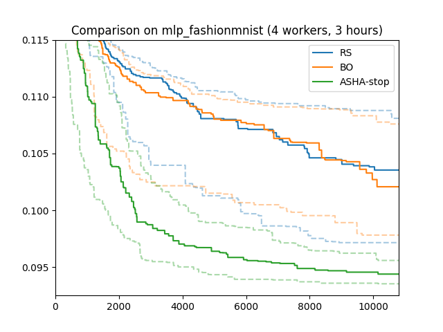
Here are results for our running example (4 workers; 3 hours; median, 25/75 percentiles over 50 repeats). ASHA stopping makes a big difference, outperforming random search and Bayesian optimization substantially. Early stopping can speed up neural network tuning dramatically, compared to standard scheduling.

If we ran for much longer, Bayesian optimization would eventually catch up with ASHA and even do better. But of course, wall-clock time matters: it is an important, if not the most important metric for automated tuning. The faster satisfying results are obtained, the more manual iterations over data, model types, and high level features can be afforded.