Bayesian Optimization
Sequential Model-Based Search
With limited parallel computing resources, experiments are sequential processes, where trials are started and report results in some ordering. This means that when deciding on which configuration to explore with any given trial, we can make use of all metric results reported by earlier trials, given that they already finished. In the simplest case, with a single worker, a new trial can start only once all earlier trials finished. We should be able to use this information in order to make better and better decisions as the experiment proceeds.
To make this precise, at any given time when a worker comes available, we need to make a decision which configuration to evaluate with the new trial, based on (a) which decisions have been made for all earlier trials, and (b) metric values reported those earlier trials which have already finished. With more than one worker, the trial set for (a) can be larger than for (b), since some trials may still be running: their results are pending. It is important to take pending trials into account, since otherwise we risk querying our objective at redundant configurations. The best way to take information (a) and (b) into account is by way of a statistical model, leading to sequential model-based decision-making.
What is the challenge for making good next configuration decisions? Say we have already evaluated the objective at a number of configurations, chosen at random. One idea is to refine the search nearby the configuration which resulted in the best metric value so far, thereby exploiting our knowledge. Even without gradients, such local search can be highly effective. On the other hand, it risks getting stuck in a local optimum. Another extreme is random search, where we explore the objective all over the search space. Choosing between these two extremes, at any given point in time, is known as explore-exploit trade-off, and is fundamental to sequential model-based search.
What is Bayesian Optimization?
One of the oldest and most widely used instantiations of sequential model-based search is Bayesian optimization. There are a number of great tutorials and review articles on Bayesian optimization, and we won’t repeat them here:
Most instances of Bayesian optimization work by modelling the objective as function \(f(\mathbf{x})\), where \(\mathbf{x}\) is a configuration from the search space. Given such a probabilistic surrogate model, we can condition it on the observed metric data (b) in order to obtain a posterior distribution. Finally, we use this posterior distribution along with additional statistics obtained from the data (such as for example the best metric value attained so far) in order to compute a acquisition function \(a(\mathbf{x})\), an (approximate) maximum of which will be our suggested configuration. While \(a(\mathbf{x})\) can itself be difficult to globally optimize, it is available in closed form and can typically be differentiated w.r.t. \(\mathbf{x}\). Moreover, it is important to understand that \(a(\mathbf{x})\) is not an approximation to \(f(\mathbf{x})\), but instead scores the expected value of sampling the objective at \(\mathbf{x}\), thereby embodying the explore-exploit trade-off. In particular, once some \(\mathbf{x}_*\) is chosen and included into the set (a), \(a(\mathbf{x}_*)\) is much diminished.
The Bayesian optimization template requires us to make two choices:
Surrogate model: By far the most common choice is to use Gaussian process surrogate models (the tutorials linked above explain the basics of Gaussian processes). A Gaussian process is parameterized by a mean and a covariance (or kernel) function. In Syne Tune, the default corresponds to what is most frequently used in practice: Matern 5/2 kernel with automatic relevance determination (ARD). A nice side effect of this choice is that the model can learn about the relative relevance of each hyperparameter as more metric data is obtained, which allows this form of Bayesian optimization to render the curse of dimensionality much less severe than it is for random search.
Acquisition function: The default choice in Syne Tune corresponds to the most popular choice in practice: expected improvement.
GP-based Bayesian optimization is run by our
launcher script
with the argument --method BO. Many options can be specified via
search_options, but we use the defaults here. See
GPFIFOSearcher for all
details. In our example, we set num_init_random to n_workers + 2, which
is the number of initial decisions made by random search, before switching
over to maximizing the acquisition function.
Results for Bayesian Optimization
|
|---|
Results for Bayesian Optimization |
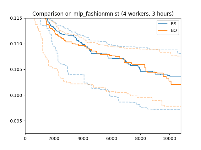
Here is how Bayesian optimization performs on our running example, compared to random search. We used the same conditions (4 workers, 3 hours experiment time, 50 random repetitions).
In this particular setup, Bayesian optimization does not outperform random search after 3 hours. This is a rather common pattern. Bayesian optimization requires a certain amount of data in order to learn enough about the objective function (in particular, about which parameters are most relevant) in order to outperform random search by targeted exploration and exploitation. If we continued to 4 or 5 hours, we would see a significant difference.
Recommendations
Here, we collect some additional recommendations. Further details are found here.
Categorical Hyperparameters
While our running example does not have any, hyperparameters of categorical type are often used. For example:
from syne_tune.config_space import lograndint, choice

config_space = {
    'n_units_1': lograndint(4, 1024),
    # ...
    'activation': choice(['ReLU', 'LeakyReLU', 'Softplus']),
}
Here, activation could determine the type of activation function.
It is important to understand that in Bayesian optimization, a
categorical parameter is encoded as vector in the multi-dimensional
unit cube: the encoding dimension is equal to the number of different
values. This is to make sure there is no ordering information between
the different values, each pair has the same distance in the encoding
space.
This is usually not what you want with numerical values, whose
ordering provide important information to the search. For example,
it sounds simpler to search over the finite range
choice([4, 8, 16, 32, 64, 128, 256, 512, 1024]) than over the infinite
lograndint(4, 1024) for n_units_1, but the opposite is the
case. The former occupies 9 dimensions, the latter 1 dimension in
the encoded space, and ordering information is lost for the former.
A better alternative is logfinrange(4, 1024, 9).
Syne Tune provides a range of finite numerical domains in order to
avoid suboptimal performance of Bayesian optimization due to the uncritical
use of choice. Since this is somewhat subtle, and you may also want
to import configuration spaces from other HPO libraries which do not
have these types, Syne Tune provides an automatic conversion logic
with streamline_config_space(). Details are given
here.
Note
When using Bayesian optimization or any other model-based HPO method,
we strongly recommend to use
streamline_config_space() in order to ensure that
your domains are chosen in a way that works best with internal encoding.
Speeding up Decision-Making
Gaussian process surrogate models have many crucial advantages over other probabilistic surrogate models typically used in machine learning. But they have one key disadvantage: inference computations scale cubically in the number of observations. For most HPO use cases, this is not a problem, since no more than a few hundred evaluations can be afforded.
Syne Tune allows to control the number of observations the GP surrogate model
is fit to, via max_size_data_for_model in search_options. If the data
is larger, it is downsampled to this size. Sampling is controlled by another
argument max_size_top_fraction. Namely, this fraction of entries in the
downsampled set are filled by those points in the full set with the best metric
values, while the remaining entries are sampled (with replacement) from the
rest of the full set. The default for max_size_data_for_model is
DEFAULT_MAX_SIZE_DATA_FOR_MODEL.
The feature is switched off by setting this to None or a very large value,
but this is not recommended. Subsampling is repeated every time the surrogate
model is fit.
Beyond, there are some search_options arguments you can use in order to
speed up Bayesian optimization. The most expensive part of making a decision
consists in refitting the parameters of the GP surrogate model, such as the ARD
parameters of the kernel. While this refitting is essential for good performance
with a small number of observations, it can be thinned out or even stopped when
the dataset gets large. You can use opt_skip_init_length,
opt_skip_period to this end (details are
here.
Warping of Inputs
If you use input_warping=True in search_options, inputs are warped
before being fed into the covariance function, the effective kernel becomes
\(k(w(x), w(x'))\), where \(w(x)\) is a warping transform with two
non-negative parameters per component. These parameters are learned along with
other parameters of the surrogate model. Input warping allows the surrogate
model to represent non-stationary functions, while still keeping the numbers
of parameters small. Note that only such components of \(x\) are warped
which belong to non-categorical hyperparameters.
Box-Cox Transformation of Target Values
This option is available only for positive target values. If you use
boxcox_transform=True in search_options, target values are transformed
before being fitted with a Gaussian marginal likelihood. This is using the Box-Cox
transform with a parameter \(\lambda\), which is learned alongside other
parameters of the surrogate model. The transform is \(\log y\) for
\(\lambda = 0\), and \(y - 1\) for \(\lambda = 1\).
Both input warping and Box-Cox transform of target values are combined in this paper:
Cowen-Rivers, A. et.al.HEBO: Pushing the Limits of Sample-efficient Hyper-parameter OptimisationJournal of Artificial Intelligence Research 74 (2022), 1269-1349
However, they fit \(\lambda\) up front by maximizing the likelihood of the targets under a univariate Gaussian assumption for the latent \(z\), while we learn \(\lambda\) jointly with all other parameters.