Using Syne Tune for Transfer Learning

Transfer learning allows us to speed up our current optimisation by learning from related optimisation runs. For instance, imagine we want to change from a smaller to a larger model. We already have a collection of hyperparameter evaluations for the smaller model. Then we can use these to guide our hyperparameter optimisation of the larger model, for instance by starting with the configuration that performed best. Or imagine that we keep the same model, but add more training data or add another data feature. Then we expect good hyperparameter configurations on the previous training data to work well on the augmented data set as well.

Syne Tune includes implementations of several transfer learning schedulers; a list of available schedulers is given here. In this tutorial we look at three of them:

  • ZeroShotTransfer
    Sequential Model-Free Hyperparameter Tuning.
    Martin Wistuba, Nicolas Schilling, Lars Schmidt-Thieme.
    IEEE International Conference on Data Mining (ICDM) 2015.

    First we calculate the rank of each hyperparameter configuration on each previous task. Then we choose configurations in order to minimise the sum of the ranks across the previous tasks. The idea is to speed up optimisation by picking configurations with high ranks on previous tasks.
  • BoundingBox
    Learning search spaces for Bayesian optimization: Another view of hyperparameter transfer learning.
    Valerio Perrone, Huibin Shen, Matthias Seeger, Cédric Archambeau, Rodolphe Jenatton.
    NeurIPS 2019.

    We construct a smaller hyperparameter search space by taking the minimum box which contains the optimal configurations for the previous tasks. The idea is to speed up optimisation by not searching areas which have been suboptimal for all previous tasks.
  • Quantiles (quantile_based_searcher)
    A Quantile-based Approach for Hyperparameter Transfer Learning.
    David Salinas, Huibin Shen, Valerio Perrone.
    ICML 2020.

    We map the hyperparameter evaluations to quantiles for each task. Then we learn a distribution of quantiles given hyperparameters. Finally, we sample from the distribution and evaluate the best sample. The idea is to speed up optimisation by searching areas with high-ranking configurations but without enforcing hard limits on the search space.

We compare them to standard BayesianOptimization (BO).

We construct a set of tasks based on the height example. We first collect evaluations on five tasks, and then compare results on the sixth. We consider the single-fidelity case. For each task we assume a budget of 10 (max_trials) evaluations. We use BO on the preliminary tasks, and for the transfer task we compare BO, ZeroShot, BoundingBox and Quantiles. The set of tasks is made by adjusting the max_steps parameter in the height example, but could correspond to adjusting the training data instead.

The code is available here. Make sure to run it as python launch_transfer_learning_example.py --generate_plots if you want to generate the plots locally. The optimisations vary between runs, so your plots might look different.

In order to run our transfer learning schedulers we need to parse the output of the tuner into a dict of TransferLearningTaskEvaluations. We do this in the extract_transferable_evaluations function.

Code to prepare evaluations from previous tasks for transfer learning.
def filter_completed(df):
    # Filter out runs that didn't finish
    return df[df["status"] == "Completed"].reset_index()


def extract_transferable_evaluations(df, metric, config_space):
    """
    Take a dataframe from a tuner run, filter it and generate
    TransferLearningTaskEvaluations from it
    """
    filter_df = filter_completed(df)

    return TransferLearningTaskEvaluations(
        configuration_space=config_space,
        hyperparameters=filter_df[config_space.keys()],
        objectives_names=[metric],
        # objectives_evaluations need to be of shape
        # (num_evals, num_seeds, num_fidelities, num_objectives)
        # We only have one seed, fidelity and objective
        objectives_evaluations=np.array(filter_df[metric], ndmin=4).T,
    )


We start by collecting evaluations by running BayesianOptimization on the five preliminary tasks. We generate the different tasks by setting max_steps=1..5 in the backend in init_scheduler, giving five very similar tasks. Once we have run BO on the task we store the evaluations as TransferLearningTaskEvaluations.

Code to initialise schedulers, use it to optimise a task and collect evaluations on preliminary tasks.
def run_scheduler_on_task(entry_point, scheduler, max_trials):
    """
    Take a scheduler and run it for max_trials on the backend specified by entry_point
    Return a dataframe of the optimisation results
    """
    tuner = Tuner(
        trial_backend=LocalBackend(entry_point=str(entry_point)),
        scheduler=scheduler,
        stop_criterion=StoppingCriterion(max_num_trials_finished=max_trials),
        n_workers=4,
        sleep_time=0.001,
    )
    tuner.run()

    return tuner.tuning_status.get_dataframe()


def init_scheduler(
    scheduler_str, max_steps, seed, mode, metric, transfer_learning_evaluations
):
    """
    Initialise the scheduler
    """
    kwargs = {
        "metric": metric,
        "config_space": height_config_space(max_steps=max_steps),
        "mode": mode,
        "random_seed": seed,
    }
    kwargs_w_trans = copy.deepcopy(kwargs)
    kwargs_w_trans["transfer_learning_evaluations"] = transfer_learning_evaluations

    if scheduler_str == "BayesianOptimization":
        return BayesianOptimization(**kwargs)

    if scheduler_str == "ZeroShotTransfer":
        return ZeroShotTransfer(use_surrogates=True, **kwargs_w_trans)

    if scheduler_str == "Quantiles":
        return FIFOScheduler(
            searcher=QuantileBasedSurrogateSearcher(**kwargs_w_trans),
            **kwargs,
        )

    if scheduler_str == "BoundingBox":
        kwargs_sched_fun = {key: kwargs[key] for key in kwargs if key != "config_space"}
        kwargs_w_trans[
            "scheduler_fun"
        ] = lambda new_config_space, mode, metric: BayesianOptimization(
            new_config_space,
            **kwargs_sched_fun,
        )
        del kwargs_w_trans["random_seed"]
        return BoundingBox(**kwargs_w_trans)
    raise ValueError("scheduler_str not recognised")


if __name__ == "__main__":

    max_trials = 10
    np.random.seed(1)
    # Use train_height backend for our tests
    entry_point = str(
        Path(__file__).parent
        / "training_scripts"
        / "height_example"
        / "train_height.py"
    )

    # Collect evaluations on preliminary tasks
    transfer_learning_evaluations = {}
    for max_steps in range(1, 6):
        scheduler = init_scheduler(
            "BayesianOptimization",
            max_steps=max_steps,
            seed=np.random.randint(100),
            mode=METRIC_MODE,
            metric=METRIC_ATTR,
            transfer_learning_evaluations=None,
        )

        print("Optimising preliminary task %s" % max_steps)
        prev_task = run_scheduler_on_task(entry_point, scheduler, max_trials)

        # Generate TransferLearningTaskEvaluations from previous task
        transfer_learning_evaluations[max_steps] = extract_transferable_evaluations(
            prev_task, METRIC_ATTR, scheduler.config_space
        )

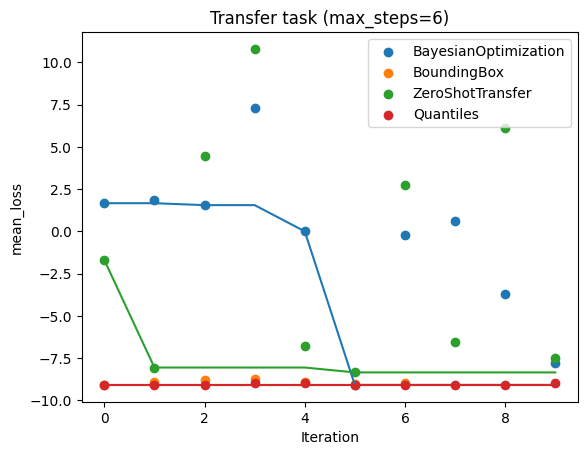
Then we run different schedulers to compare on our transfer task with max_steps=6. For ZeroShotTransfer we set use_surrogates=True, meaning that it uses an XGBoost model to estimate the rank of configurations, as we do not have evaluations of the same configurations on all previous tasks.

Code to run schedulers on transfer task.
    # Collect evaluations on transfer task
    max_steps = 6
    transfer_task_results = {}
    labels = ["BayesianOptimization", "BoundingBox", "ZeroShotTransfer", "Quantiles"]
    for scheduler_str in labels:
        scheduler = init_scheduler(
            scheduler_str,
            max_steps=max_steps,
            seed=max_steps,
            mode=METRIC_MODE,
            metric=METRIC_ATTR,
            transfer_learning_evaluations=transfer_learning_evaluations,
        )
        print("Optimising transfer task using %s" % scheduler_str)
        transfer_task_results[scheduler_str] = run_scheduler_on_task(
            entry_point, scheduler, max_trials
        )

We plot the results on the transfer task. We see that the early performance of the transfer schedulers is much better than standard BO. We only plot the first max_trials results. The transfer task is very similar to the preliminary tasks, so we expect the transfer schedulers to do well. And that is what we see in the plot below.

Plotting helper code.
def add_labels(ax, conf_space, title):
    ax.legend()
    ax.set_xlabel("width")
    ax.set_ylabel("height")
    ax.set_xlim([conf_space["width"].lower - 1, conf_space["width"].upper + 1])
    ax.set_ylim([conf_space["height"].lower - 10, conf_space["height"].upper + 10])
    ax.set_title(title)


def scatter_space_exploration(ax, task_hyps, max_trials, label, color=None):
    ax.scatter(
        task_hyps["width"][:max_trials],
        task_hyps["height"][:max_trials],
        alpha=0.4,
        label=label,
        color=color,
    )


colours = {
    "BayesianOptimization": "C0",
    "BoundingBox": "C1",
    "ZeroShotTransfer": "C2",
    "Quantiles": "C3",
}


def plot_last_task(max_trials, df, label, metric, color):
    max_tr = min(max_trials, len(df))
    plt.scatter(range(max_tr), df[metric][:max_tr], label=label, color=color)
    plt.plot([np.min(df[metric][:ii]) for ii in range(1, max_trials + 1)], color=color)


Code to plot results on transfer task.
    # Optionally generate plots. Defaults to False
    parser = argparse.ArgumentParser()
    parser.add_argument(
        "--generate_plots", action="store_true", help="generate optimisation plots."
    )
    args = parser.parse_args()

    if args.generate_plots:
        from syne_tune.try_import import try_import_visual_message

        try:
            import matplotlib.pyplot as plt
        except ImportError:
            print(try_import_visual_message())

        print("Generating optimisation plots.")
        """ Plot the results on the transfer task """
        for label in labels:
            plot_last_task(
                max_trials,
                transfer_task_results[label],
                label=label,
                metric=METRIC_ATTR,
                color=colours[label],
            )
        plt.legend()
        plt.ylabel(METRIC_ATTR)
        plt.xlabel("Iteration")
        plt.title("Transfer task (max_steps=6)")
        plt.savefig("Transfer_task.png", bbox_inches="tight")
../../_images/Transfer_task.png

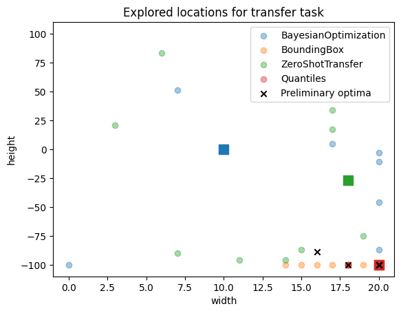
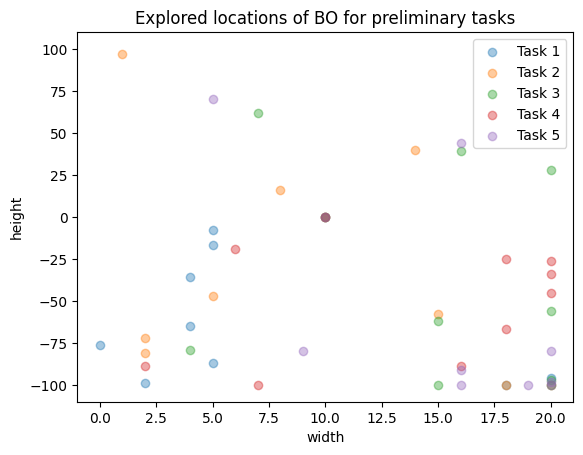
We also look at the parts of the search space explored. First by looking at the preliminary tasks.

Code to plot the configurations tried for the preliminary tasks.
        """ Plot the configs tried for the preliminary tasks """
        fig, ax = plt.subplots()
        for key in transfer_learning_evaluations:
            scatter_space_exploration(
                ax,
                transfer_learning_evaluations[key].hyperparameters,
                max_trials,
                "Task %s" % key,
            )
        add_labels(
            ax,
            scheduler.config_space,
            "Explored locations of BO for preliminary tasks",
        )
        plt.savefig("Configs_explored_preliminary.png", bbox_inches="tight")
../../_images/Configs_explored_preliminary.png

Then we look at the explored search space for the transfer task. For all the transfer methods the first tested point (marked as a square) is closer to the previously explored optima (in black crosses), than for BO which starts by checking the middle of the search space.

Code to plot the configurations tried for the transfer task.
        """ Plot the configs tried for the transfer task """
        fig, ax = plt.subplots()

        # Plot the configs tried by the different schedulers on the transfer task
        for label in labels:
            finished_trials = filter_completed(transfer_task_results[label])
            scatter_space_exploration(
                ax, finished_trials, max_trials, label, color=colours[label]
            )

            # Plot the first config tested as a big square
            ax.scatter(
                finished_trials["width"][0],
                finished_trials["height"][0],
                marker="s",
                color=colours[label],
                s=100,
            )

        # Plot the optima from the preliminary tasks as black crosses
        past_label = "Preliminary optima"
        for key in transfer_learning_evaluations:
            argmin = np.argmin(
                transfer_learning_evaluations[key].objective_values(METRIC_ATTR)[
                    :max_trials, 0, 0
                ]
            )
            ax.scatter(
                transfer_learning_evaluations[key].hyperparameters["width"][argmin],
                transfer_learning_evaluations[key].hyperparameters["height"][argmin],
                color="k",
                marker="x",
                label=past_label,
            )
            past_label = None
        add_labels(ax, scheduler.config_space, "Explored locations for transfer task")
        plt.savefig("Configs_explored_transfer.png", bbox_inches="tight")
../../_images/Configs_explored_transfer.png