Comparing Different HPO Methods
We have learned about different methods for hyperparameter tuning:
RandomSearch: Sample configurations at randomBayesianOptimization: Learn how to best sample by probabilistic modeling of past observationsASHA: Compare running trials with each other after certain numbers of epochs and stop those which underperformMOBSTER: Combine early stopping fromASHAwith informed sampling fromBayesianOptimization
How do these methods compare when applied to our transformer_wikitext2 tuning
problem? In this section, we look at comparative plots which can easily be
generated with Syne Tune.
Note
Besides MOBSTER, Syne Tune provides
a number of additional state-of-the-art model-based variants of
ASHA, such as
HyperTune or
DyHPO. Moreover, these methods can
be configured in many ways, see
this tutorial.
A Comparative Study
It is easy to compare different setups with each other in Syne Tune, be it a number of HPO methods, or the same method on different variations, such as different number of workers, or different configuration spaces. First, we specify which methods to compare with each other:
from syne_tune.experiments.default_baselines import (
    RandomSearch,
    BayesianOptimization,
    ASHA,
    MOBSTER,
)


class Methods:
    RS = "RS"
    BO = "BO"
    ASHA = "ASHA"
    MOBSTER = "MOBSTER"


methods = {
    Methods.RS: lambda method_arguments: RandomSearch(method_arguments),
    Methods.BO: lambda method_arguments: BayesianOptimization(method_arguments),
    Methods.ASHA: lambda method_arguments: ASHA(method_arguments, type="promotion"),
    Methods.MOBSTER: lambda method_arguments: MOBSTER(
        method_arguments, type="promotion"
    ),
}
We compare random search (RS), Bayesian Optimization (BO), ASHA
(ASHA), and MOBSTER (MOBSTER), deviating from the defaults for
each method only in that we use the promotion (or pause-and-resume)
variant of the latter two. Next, we specify which baselines we would like
to consider in our study:
from typing import Dict

from syne_tune.experiments.benchmark_definitions import RealBenchmarkDefinition
from transformer_wikitext2.code.transformer_wikitext2_definition import (
    transformer_wikitext2_benchmark,
)


def benchmark_definitions(
    sagemaker_backend: bool = False, **kwargs
) -> Dict[str, RealBenchmarkDefinition]:
    return {
        "transformer_wikitext2": transformer_wikitext2_benchmark(
            sagemaker_backend=sagemaker_backend, **kwargs
        ),
    }
The only benchmark we consider in this study is our transformer_wikitext2
tuning problem, with its default configuration space (in general, many
benchmarks can be selected from
benchmarking.benchmark_definitions.real_benchmark_definitions.real_benchmark_definitions()).
Our study has the following properties:
We use
LocalBackendas execution backend, which runsn_workers=4trials as parallel processes. The AWS instance type isinstance_type="ml.g4dn.12xlarge", which provides 4 GPUs, one for each worker.We repeat each experiment 10 times with different random seeds, so that all in all, we run 40 experiments (4 methods, 10 seeds).
These details are specified in scripts
hpo_main.py and
launch_remote.py, which we will
discuss in more detail in Module 2, along with the
choice of the execution backend. Once all experiments have finished (if all of
them are run in parallel, this takes a little more than max_wallclock_time,
or 5 hours), we can visualize results.
|
|---|
Comparison of methods on transformer_wikitext2 benchmark, using the local backend with 4 workers. |
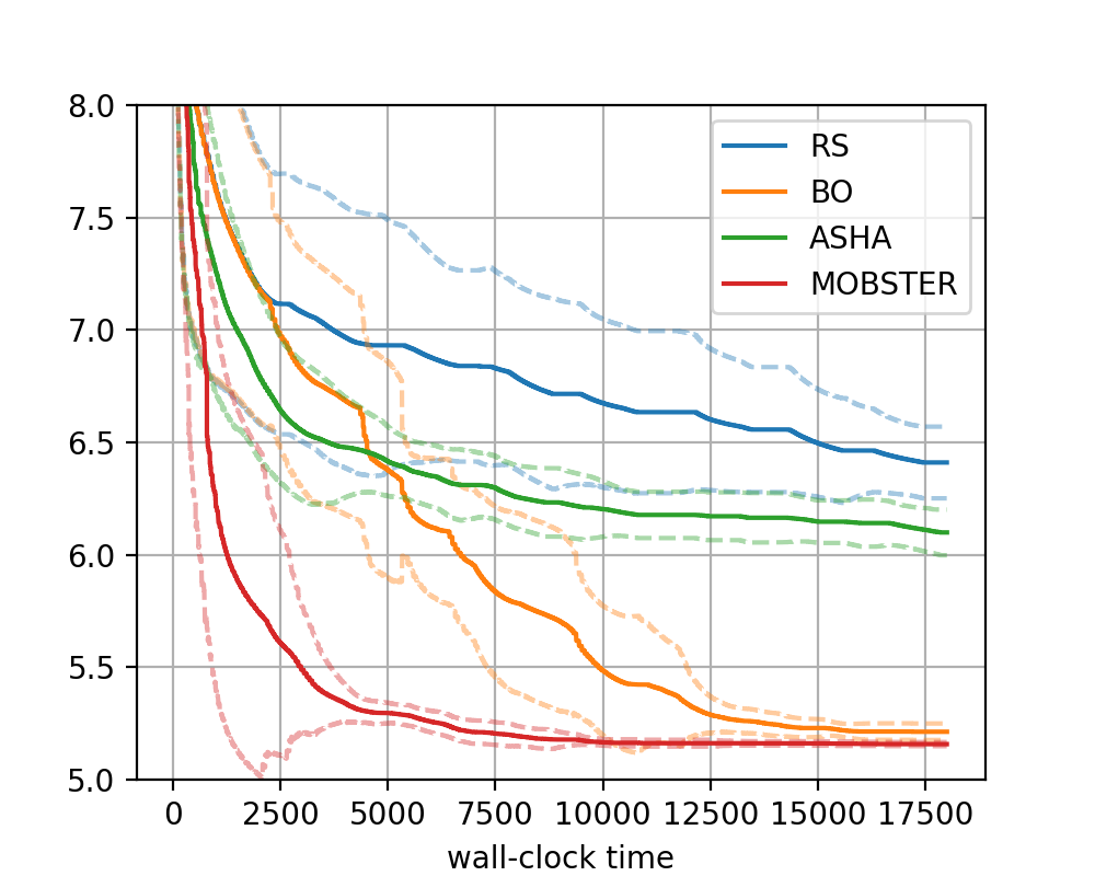
We can clearly see the benefits coming both from Bayesian optimization
(intelligent rather than random sampling) and multi-fidelity scheduling. A
combination of the two, MOBSTER, provides both a rapid initial decrease
and the best performance after 5 hours.