Visualization of Results
Once all results are obtained, we would rapidly like to create comparative plots.
In Syne Tune, each experiment stores two files, metadata.json with metadata,
and results.csv.zip containing time-stamped results. The
Tuner object at the end of the experiment is also serialized
to tuner.dill, but this is not needed here.
Note
This section offers an example of the plotting facilities in Syne Tune. More details are provided in this tutorial.
First, we need to download the results from S3 to the local disk. This can be
done by a command which is also printed at the end of launch_remote.py:
aws s3 sync s3://<BUCKET-NAME>/syne-tune/docs-2/ ~/syne-tune/docs-2/ \
  --exclude "*" --include "*metadata.json" --include "*results.csv.zip"
This command can also be run from inside the plotting code. Note that the
tuner.dill result files are not downloaded, since they are not needed for
result visualization.
Here is the code for generating result plots for two of the benchmarks:
from typing import Dict, Any, Optional, List, Set
import logging

from baselines import methods
from benchmark_definitions import benchmark_definitions
from hpo_main import RungLevelsExtraResults
from syne_tune.experiments import ComparativeResults, PlotParameters, SubplotParameters


def metadata_to_setup(metadata: Dict[str, Any]) -> Optional[str]:
    # The setup is the algorithm. No filtering
    return metadata["algorithm"]


SETUP_TO_SUBPLOT = {
    "ASHA": 0,
    "MOBSTER": 0,
    "ASHA-TANH": 1,
    "MOBSTER-TANH": 1,
    "ASHA-RELU": 2,
    "MOBSTER-RELU": 2,
    "RS": 3,
    "BO": 3,
}


def metadata_to_subplot(metadata: Dict[str, Any]) -> Optional[int]:
    return SETUP_TO_SUBPLOT[metadata["algorithm"]]


def _print_extra_results(
    extra_results: Dict[str, Dict[str, List[float]]],
    keys: List[str],
    skip_setups: Set[str],
):
    for setup_name, results_for_setup in extra_results.items():
        if setup_name not in skip_setups:
            print(f"[{setup_name}]:")
            for key in keys:
                values = results_for_setup[key]
                print(f"  {key}: {[int(x) for x in values]}")


if __name__ == "__main__":
    logging.getLogger().setLevel(logging.INFO)
    experiment_name = "docs-2"
    experiment_names = (experiment_name,)
    setups = list(methods.keys())
    num_runs = 20
    download_from_s3 = False  # Set ``True`` in order to download files from S3
    # Plot parameters across all benchmarks
    plot_params = PlotParameters(
        xlabel="wall-clock time",
        aggregate_mode="iqm_bootstrap",
        grid=True,
    )
    # We would like four subplots (2 row, 2 columns), each showing two setups.
    # Each subplot gets its own title, and legends are shown in each,
    plot_params.subplots = SubplotParameters(
        nrows=2,
        ncols=2,
        kwargs=dict(sharex="all", sharey="all"),
        titles=[
            "activations tuned",
            "activations = tanh",
            "activations = relu",
            "single fidelity",
        ],
        title_each_figure=True,
        legend_no=[0, 1, 2, 3],
    )

    # The creation of ``results`` downloads files from S3 (only if
    # ``download_from_s3 == True``), reads the metadata and creates an inverse
    # index. If any result files are missing, or there are too many of them,
    # warning messages are printed
    results = ComparativeResults(
        experiment_names=experiment_names,
        setups=setups,
        num_runs=num_runs,
        metadata_to_setup=metadata_to_setup,
        plot_params=plot_params,
        metadata_to_subplot=metadata_to_subplot,
        download_from_s3=download_from_s3,
    )

    # We can now create plots for the different benchmarks:
    # - We store the figures as PNG files
    # - We also load the extra results collected during the experiments
    #   (recall that we monitored sizes of rungs for ASHA and MOBSTER).
    #   Instead of plotting their values over time, we print out their
    #   values at the end of each experiment
    extra_results_keys = RungLevelsExtraResults().keys()
    skip_setups = {"RS", "BO"}
    # First: fcnet-protein
    benchmark_name = "fcnet-protein"
    benchmark = benchmark_definitions[benchmark_name]
    # These parameters overwrite those given at construction
    plot_params = PlotParameters(
        metric=benchmark.metric,
        mode=benchmark.mode,
        ylim=(0.22, 0.30),
    )
    extra_results = results.plot(
        benchmark_name=benchmark_name,
        plot_params=plot_params,
        file_name=f"./{experiment_name}-{benchmark_name}.png",
        extra_results_keys=extra_results_keys,
    )["extra_results"]
    _print_extra_results(extra_results, extra_results_keys, skip_setups=skip_setups)
    # Next: fcnet-slice
    benchmark_name = "fcnet-slice"
    benchmark = benchmark_definitions[benchmark_name]
    # These parameters overwrite those given at construction
    plot_params = PlotParameters(
        metric=benchmark.metric,
        mode=benchmark.mode,
        ylim=(0.00025, 0.0012),
    )
    results.plot(
        benchmark_name=benchmark_name,
        plot_params=plot_params,
        file_name=f"./{experiment_name}-{benchmark_name}.png",
        extra_results_keys=extra_results_keys,
    )
    _print_extra_results(extra_results, extra_results_keys, skip_setups=skip_setups)
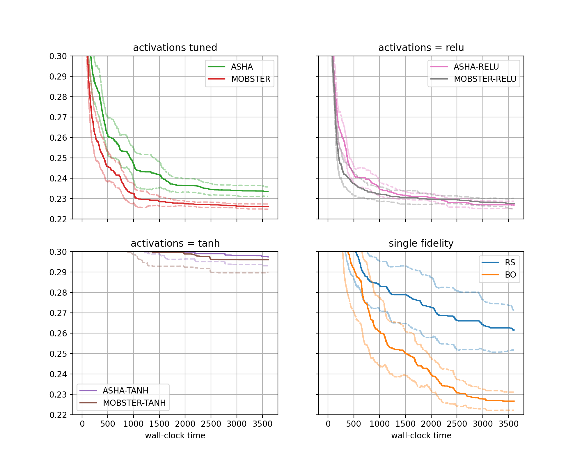
The figure for benchmark fcnet-protein looks as follows:
|
|---|
Results for FCNet (protein dataset) |
Moreover, we obtain an output for extra results, as follows:
[ASHA]:
  num_at_level1: [607, 630, 802, 728, 669, 689, 740, 610, 566, 724, 691, 812, 837, 786, 501, 642, 554, 625, 531, 672]
  num_at_level3: [234, 224, 273, 257, 247, 238, 271, 222, 191, 256, 240, 273, 287, 272, 185, 227, 195, 216, 197, 241]
  num_at_level9: [97, 81, 99, 95, 99, 99, 106, 92, 73, 98, 90, 95, 99, 98, 74, 86, 78, 82, 85, 101]
  num_at_level27: [49, 36, 37, 36, 41, 47, 37, 43, 36, 35, 34, 37, 39, 39, 39, 44, 41, 30, 45, 49]
  num_at_level81: [22, 17, 18, 15, 21, 22, 19, 26, 20, 15, 16, 13, 13, 23, 27, 29, 20, 17, 20, 26]
[MOBSTER]:
  num_at_level1: [217, 311, 310, 353, 197, 96, 377, 135, 364, 336, 433, 374, 247, 282, 175, 302, 187, 225, 182, 240]
  num_at_level3: [107, 133, 124, 138, 104, 64, 163, 72, 157, 132, 146, 140, 123, 112, 110, 129, 90, 100, 86, 126]
  num_at_level9: [53, 62, 55, 59, 66, 51, 83, 47, 72, 55, 54, 59, 54, 51, 72, 65, 60, 49, 55, 70]
  num_at_level27: [29, 34, 30, 26, 50, 37, 49, 31, 27, 25, 23, 28, 27, 28, 49, 33, 42, 27, 34, 45]
  num_at_level81: [18, 20, 16, 14, 33, 25, 37, 24, 13, 17, 10, 14, 17, 20, 32, 24, 29, 15, 26, 31]
[ASHA-TANH]:
  num_at_level1: [668, 861, 755, 775, 644, 916, 819, 710, 694, 870, 764, 786, 769, 710, 862, 807, 859, 699, 757, 794]
  num_at_level3: [237, 295, 265, 272, 221, 311, 302, 246, 246, 294, 278, 280, 276, 240, 297, 290, 304, 258, 270, 279]
  num_at_level9: [86, 112, 101, 97, 91, 104, 119, 90, 92, 104, 98, 96, 98, 90, 108, 120, 105, 109, 105, 102]
  num_at_level27: [37, 47, 39, 39, 40, 39, 45, 44, 39, 41, 41, 44, 44, 40, 45, 43, 38, 53, 49, 39]
  num_at_level81: [21, 16, 16, 16, 20, 16, 17, 18, 17, 14, 18, 21, 21, 20, 17, 19, 16, 19, 23, 20]
[MOBSTER-TANH]:
  num_at_level1: [438, 594, 462, 354, 307, 324, 317, 359, 483, 523, 569, 492, 516, 391, 408, 565, 492, 322, 350, 479]
  num_at_level3: [166, 206, 156, 135, 133, 127, 129, 131, 175, 211, 191, 165, 178, 169, 151, 204, 164, 122, 132, 205]
  num_at_level9: [69, 75, 56, 54, 78, 60, 57, 60, 76, 80, 72, 56, 72, 103, 67, 77, 63, 48, 59, 92]
  num_at_level27: [36, 35, 25, 28, 45, 37, 27, 36, 46, 27, 37, 26, 37, 58, 31, 36, 26, 28, 33, 39]
  num_at_level81: [20, 13, 12, 11, 23, 20, 13, 20, 23, 10, 13, 9, 18, 31, 16, 18, 11, 16, 19, 21]
[ASHA-RELU]:
  num_at_level1: [599, 670, 682, 817, 608, 585, 770, 397, 613, 721, 599, 601, 618, 718, 613, 674, 715, 638, 598, 652]
  num_at_level3: [201, 246, 242, 277, 225, 209, 282, 140, 212, 245, 202, 205, 215, 245, 207, 239, 238, 224, 221, 234]
  num_at_level9: [75, 94, 94, 100, 89, 92, 101, 60, 78, 89, 76, 82, 80, 98, 86, 96, 83, 84, 90, 91]
  num_at_level27: [37, 43, 36, 34, 40, 45, 39, 35, 34, 31, 40, 40, 38, 39, 35, 34, 29, 34, 41, 35]
  num_at_level81: [23, 19, 14, 13, 19, 21, 15, 24, 17, 13, 20, 18, 19, 18, 20, 16, 13, 15, 22, 17]
[MOBSTER-RELU]:
  num_at_level1: [241, 319, 352, 438, 354, 386, 197, 262, 203, 387, 320, 139, 359, 401, 334, 294, 361, 403, 178, 141]
  num_at_level3: [110, 156, 135, 166, 138, 143, 104, 124, 95, 136, 133, 71, 133, 151, 130, 122, 134, 151, 92, 74]
  num_at_level9: [50, 83, 59, 75, 59, 55, 57, 72, 53, 53, 58, 40, 62, 63, 61, 54, 52, 65, 48, 47]
  num_at_level27: [31, 51, 29, 31, 29, 23, 39, 38, 36, 20, 29, 36, 32, 29, 32, 29, 24, 27, 31, 34]
  num_at_level81: [20, 35, 12, 11, 12, 15, 22, 18, 26, 12, 16, 27, 16, 15, 20, 15, 15, 13, 18, 22]
There are four subfigures arranged as two-by-two matrix. Each contains two curves in bold, along with confidence intervals. The horizontal axis depicts wall-clock time, and on the vertical axis, we show the best metric value found until this time.
More general, the data from our 640 experiments can be grouped w.r.t. subplot, then setup. Each setup gives rise to one curve (bold, with confidence band). Subplots are optional, the default is to plot a single figure.
The function
metadata_to_setupmaps the metadata stored for an experiment to the setup name. In our basic case, the setup is simply the name of the method.The function
metadata_to_subplotmaps the metadata to the subplot index (0, 1, 2, 3). We group setups with the same configuration space, but also split multi-fidelity and single-fidelity methods.Once the data is grouped w.r.t. benchmark, then subplot (optional), then setup, we should be left with 20 experiments, one for each seed. These 20 curves are now interpolated to a common grid, and at each grid point, the 20 values are aggregated into
lower,aggregate,upper. In the figure,aggregateis shown in bold, andlower,upperin dashed. Different aggregation modes are supported (selected byplot_params.aggregate_mode).We pass
extra_results_keysto theplot()method in order to also retrieve extra results. This method returns a dictionary, whose “extra_results” entry is what we need.
Advanced Experimenting
Once you start to run many experiments, you will get better at avoiding wasteful repetitions. Here are some ways in which Syne Tune can support you.
Combining results from several studies: It often happens that results for a new idea need to be compared to baselines on a common set of benchmarks. You do not have to re-run baselines, but can easily combine older results with more recent ones. This is explained here.
When running many experiments, some may fail. Syne Tune supports you in not having to re-run everything from scratch. As already noted above, when creating aggregate plots, it is important not to use incomplete results stored for failed experiments. The cleanest way to do so is to remove these results on S3. Another option is to filter out corrupt results:
If you forget about removing such corrupt results, you will get a reminder when creating
ComparativeResults. Since you pass the list of setup names and the number of seeds (innum_runs), you get a warning when too many experiments have been found, along with the path names.Results are stored on S3, using object name prefixes of the form
<s3-bucket>/syne-tune/docs-2/ASHA/docs-2-fcnet-protein-7-2023-04-20-15-20-18-456/or<s3-bucket>/syne-tune/docs-2/MOBSTER-7/docs-2-fcnet-protein-7-2023-04-20-15-20-00-677/. The pattern is<tag>/<method>/<tag>-<benchmark>-<seed>-<datetime>/for cheap methods, and<tag>/<method>-<seed>/<tag>-<benchmark>-<seed>-<datetime>/for expensive methods.Instead of removing corrupt results on S3, you can also filter them by datetime, using the
datetime_boundsargument ofComparativeResults. This allows you define an open or closed datetime range for results you want to keep. If your failed attempts preceed the ones that finally worked out, this type of filtering can save you the head-ache of removing files on S3.Warning: When you remove objects on S3 for some experiment tag, it is strongly recommended to remove all result files locally (so everything at
~/syne-tune/<tag>/) and sync them back from S3, using the command at the start of this section.aws s3 syncis prone to make mistakes otherwise, which are very hard to track down.