Synchronous Successive Halving and Hyperband
In this section, we will introduce some simple multi-fidelity HPO methods based on synchronous decision-making. Methods discussed here are not model-based, they suggest new configurations simply by drawing them uniformly at random from the configuration space, much like random search does.
Early Stopping Hyperparameter Configurations
The figure below depicts learning curves of a set of neural networks with different hyperparameter configurations trained for the same number of epochs. After a few epochs we are already able to visually distinguish between the well-performing and the poorly performing ones. However, the ordering is not perfect, and we might still require the full amount of 100 epochs to identify the best performing configuration.
|
|---|
Learning curves for randomly drawn hyperparameter configurations |
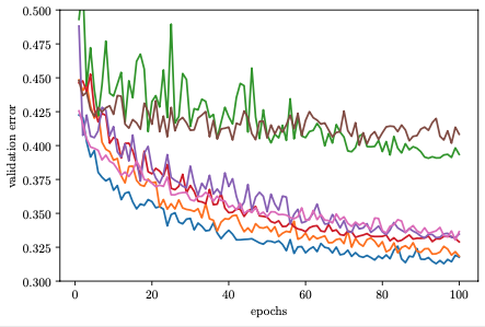
The idea of early stopping based HPO methods is to free up compute resources by early stopping the evaluation of poorly performing configurations and allocate them to more promising ones. This speeds up the optimization process, since we have a higher throughput of configurations that we can try.
Recall the notation of resource from the introduction. In this tutorial, resource equates to epochs trained, so \(r=2\) refers to metric values evaluated at the end of the second epoch. The main objective of interest, validation error in our tutorial, is denoted by \(f(\mathbf{x}, r)\), where \(\mathbf{x}\) is the configuration, \(r\) the resource level. Our problem typically defines a maximum resource level \(r_{max}\), so that in general the goal is to find \(\mathbf{x}\) which minimizes \(f(\mathbf{x}, r_{max})\). In NASBench-201, the maximum number of epochs is \(r_{max} = 200\).
Synchronous Successive Halving
One of the simplest competitive multi-fidelity HPO methods is synchronous successive halving (SH). The basic idea is to start with \(N\) configurations randomly sampled from the configuration space, training each of them for \(r_{min}\) epochs only (e.g., \(r_{min} = 1\)). We then discard a fraction of the worst performing trials and train the remaining ones for longer. Iterating this process, fewer trials run for longer, until at least one trial reaches \(r_{max}\) epochs.
More formally, successive halving (SH) is parameterized by a minimum resource \(r_{min}\) (for example 1 epoch) and a halving constant \(\eta\in\{2, 3, \dots\}\). The defaults in Syne Tune are \(r_{min} = 1\) and \(\eta = 3\), and we will use these for now. Next, we define rung levels \(\mathcal{R} = \{ r_{min}, r_{min}\eta, r_{min}\eta^2, \dots \}\), so that all \(r\in \mathcal{R}\) satisfy \(r\le r_{max}\). In our example, \(\mathcal{R} = \{ 1, 3, 9, 27, 81 \}\). Moreover, the initial number of configurations is set to \(N = \eta^5 = 243\). In general, a trial is trained until reaching the next recent rung level, then evaluated there, and the validation errors of all trials at a rung level are used to decide which of them to discard. We start with running \(N\) trials until rung level \(r_{min}\). Sorting the validation errors, we keep the top \(1 / \eta\) fraction (i.e, \(N / \eta\) configurations) and discard all the rest. The surviving trials are trained for \(r_{min}\eta\) epochs, and the process is repeated. Synchronized at each rung level, a \(1 / \eta\) fraction of trials survives and finds it budget to be multiplied by \(\eta\). With this particular choice of \(N\), only a single trial will be trained to the full resource \(r_{max}\). In our example:
We first train 243 randomly chosen configurations for 1 epoch each
Once all of them are finished, we promote those 81 trials with the lowest validation errors to train for 3 epochs
Then, the 27 best-performing ones after 3 epochs are trained for 9 epochs
The 9 best ones after 9 epochs are trained for 27 epochs
The 3 best ones after 27 epochs are trained for 81 epochs
The single best configuration after 81 epochs is trained for 200 epochs
Finally, once one such round of SH is finished, we start the next round with a new set of initial configurations, until the total budget is spent.
Our launcher script runs synchronous
successive halving if method="SYNCSH". The relevant parameters are
grace_period ( \(r_{min}\) ) and reduction_factor ( \(\eta\) ).
Moreover, for SH, we need to set brackets=1, since otherwise an extension
called Hyperband is run (to be discussed shortly).
API docs:
Baseline:
SyncHyperbandAdditional arguments:
SynchronousGeometricHyperbandScheduler
Synchronous SH employs pause-and-resume scheduling (see introduction). Once a trial reaches a rung level, it is paused there. This is because the decision of which trials to promote to the next rung level can only be taken once the current rung level is completely filled up: only then can we determine the top \(1 / \eta\) fraction of trials which are to be resumed. Syne Tune supports pause-and-resume schedulers with checkpointing. Namely, the state of a trial (e.g., weights of neural network model) is stored when it is paused. Once a trial is resumed, the checkpoint is loaded and training can resume from there. Say a trial is paused at \(r = 9\) and is later resumed towards \(r = 27\). With checkpointing, we have to train for \(27 - 9 = 18\) epochs only instead of 27 epochs for training from scratch. More details are given here. For tabulated benchmarks, checkpointing is supported by default.
Finally, it is important to understand in which sense the method detailed in this section is synchronous. This is because decision-making on which trials to resume is synchronized at certain points in time, namely when a rung level is completed. In general, a trial reaching a rung level has to be paused, because it is not the last one required to fill the rung. In our example, the rung at \(r = 1\) requires 243 trials to finish training for one epoch, so that 242 of them have to be paused for some time.
Synchronous decision-making does not mean that parallel compute resources (called workers in Syne Tune) need to sit idle. In Syne Tune, workers are asychronously scheduled in general: whenever a worker finishes, it is assigned a new task immediately. Say a worker just finished, but we find all remaining slots in the current rung to be pending (meaning that other workers evaluate trials to end up there, but are not finished yet). We cannot resume a trial from this rung, because promotion decisions require all slots to be filled. In such cases, our implementation starts a new round of SH (or further contributes to a new round already started for the same reason).
In the sequel, the synchronous / asynchronous terminology always refers to decision-making, and not to scheduling of parallel resources.
Synchronous Hyperband
While SH can greatly improve upon random search, the choice of \(r_{min}\) can have an impact on its performance. If \(r_{min}\) is too small, our network might not have learned anything useful, and even the best configurations may be filtered out at random. If \(r_{min}\) is too large on the other hand, the benefits of early stopping may be greatly diminished.
Hyperband is an extension of SH that mitigates the risk of setting \(r_{min}\) too small. It runs SH as subroutine, where each round, called a bracket, balances between \(r_{min}\) and the number of initial configurations \(N\), such that the same total amount of resources is used. One round of Hyperband consists of a sequential loop over brackets.
The number of brackets can be chosen anywhere between 1 (i.e., SH) and the number of rung levels. In Syne Tune, the default number of brackets is the maximum. Without going into formal details, here are the brackets for our NASBench-201 example:
Bracket 0: \(r_{min} = 1, N = 243\)
Bracket 1: \(r_{min} = 3, N = 98\)
Bracket 2: \(r_{min} = 9, N = 41\)
Bracket 3: \(r_{min} = 27, N = 18\)
Bracket 4: \(r_{min} = 81, N = 9\)
Bracket 5: \(r_{min} = 200, N = 6\)
Our launcher script runs synchronous
Hyperband if method="SYNCHB". Since brackets is not used when creating
SyncHyperband, the maximum value 6 is chosen. We also use the default
values for grace_period (1) and reduction_factor (3).
API docs:
Baseline:
SyncHyperbandAdditional arguments:
SynchronousGeometricHyperbandScheduler
The advantages of Hyperband over SH are mostly theoretical. In practice, while Hyperband can improve on SH if \(r_{min}\) chosen for SH is clearly too small, it tends to perform worse than SH if \(r_{min}\) is adequate. This disadvantage of Hyperband is somewhat mitigated in the Syne Tune implementation, where new brackets are started whenever workers cannot contribute to the current bracket (because remaining slots in the current rung are pending, see above).